Having established in my previous post that softmax looks like the way to go for my final activation layer it’s time to think about the cost function. And this one is trickier.

Hypothesis: Use Mean Squared Error Cost Function

The standard cost function for multi-class classifiers is usually categorical cross-entropy. But I don’t think that’s the right way to go for what I’m building. Here’s the equation:\(\)

$$-\frac{1}{m}\sum\limits_{i = 1}^{m} (y^{(i)}\log\left(a^{[L] (i)}\right) + (1-y^{(i)})\log\left(1- a^{[L](i)}\right))$$

This makes complete sense in a standard supervised learning context when the label values will all be either 0 or 1. In that context, we realize that in practice, this is really two equations. In situations where \(y = 1\) the equation becomes:

$$-\frac{1}{m}\sum\limits_{i = 1}^{m} (y^{(i)}\log\left(a^{[L] (i)}\right))$$

And when \(y = 0\) we have:

$$-\frac{1}{m}\sum\limits_{i = 1}^{m} ((1-y^{(i)})\log\left(1- a^{[L](i)}\right))$$

But so what? Well, here’s where the particulars of how I need to implement this becomes an issue. You see, unlike a standard supervised learning problem, I need to accommodate more than just \(y = 0,1\). As mentioned in the last post, I’m generating softmax values for 48 output nodes:

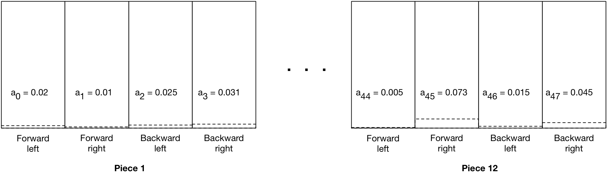
And for sure, the labels for some of those outputs will be classical supervised learning labels. Specifically, every board state has moves that are legal and those that are not. Illegal moves will be reinforced as such by training the model with zero labels for each illegal move.

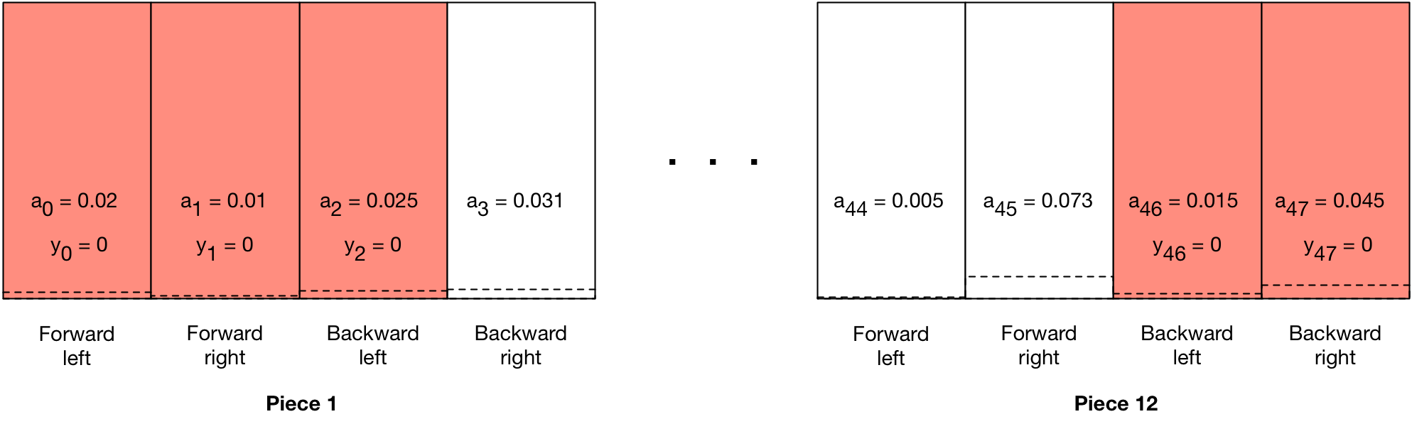
This will have the effect of creating a gradient for each illegal move that pulls the activation value down towards zero, decreasing the probability of “predicting” (to use the classifier term) that move next time around. This will be an unambiguous signal to the network since an illegal move is entirely deterministic based on board state.

Training to make successful moves is a little more subtle. Here, in a game, for each board state of the game, the model will generate its probabilistic estimate of the best move. That probability will be used to pick the actual move made (“roll the dice”), and the actual move made will become a “fake label.” If the move was ultimately part of a winning game, it will be assigned a label \(y = 1\):

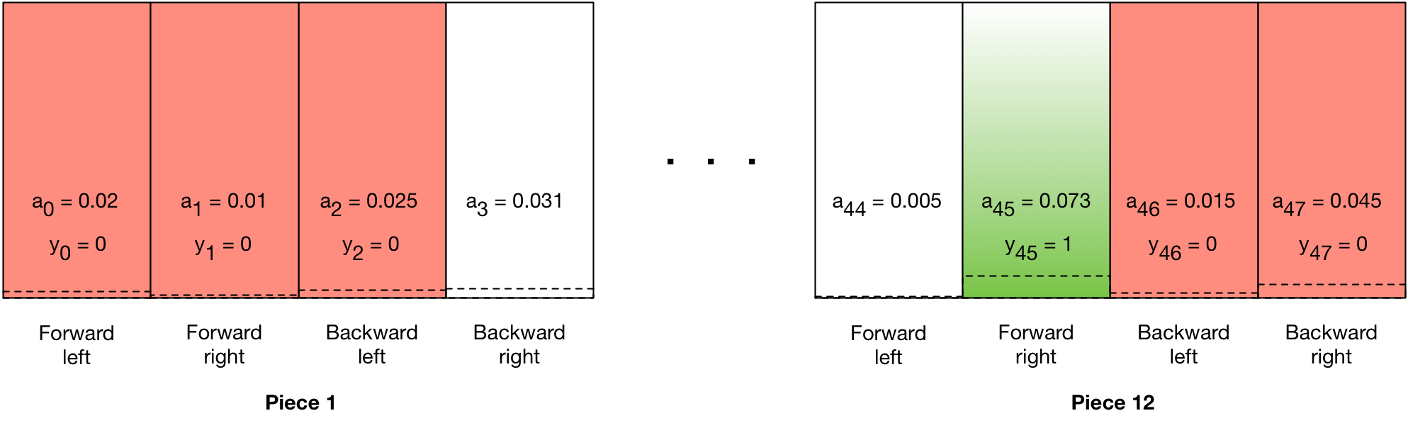
This will have the effect of creating a gradient that pushes the probability of that move higher in subsequent games with that board state. If the same move, however, was part of a losing game, it will be assigned a fake label \(y = 0\):

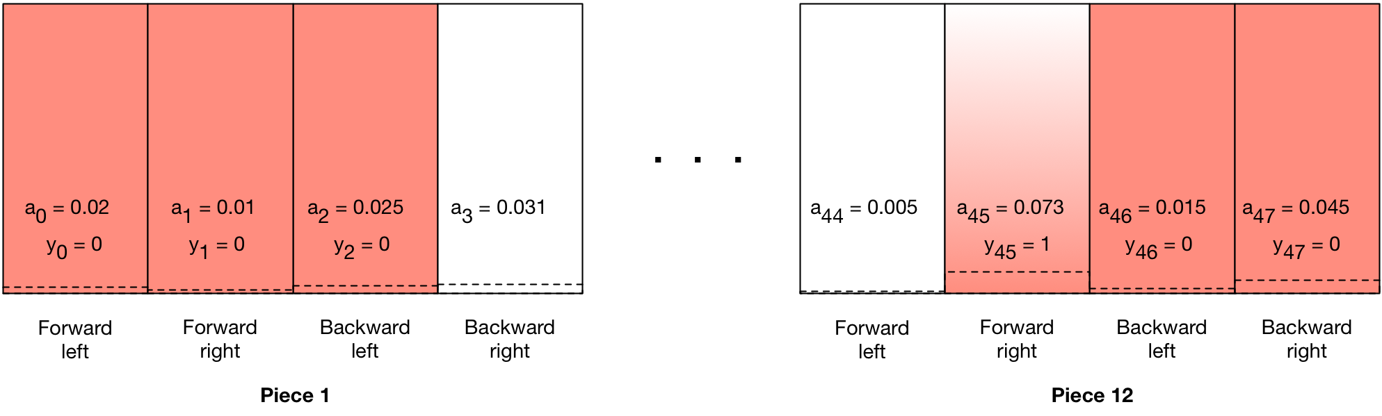
This will have the effect of pushing the probability of that move lower in subsequent games with that board state. In fact the exact same board state / move combination could result in a win in one game, and a loss in another. And unlike the illegal moves reinforcement, the actual \(Y\) value will be discounted the farther away the move was from the actual win.

So what does all this have to do with the cost function?

Good question. We’ve already seen that the label will be discounted from either \(Y = 1\) or \(Y = 0\) which means that the cost function that will be optimized for values that aren’t exactly 1 or 0. That might not necessarily be a big deal, but what about the labels where it’s not an illegal move or a discounted actual move, win or loss? That is, the possible legal moves that were not actually taken. My hypothesis is that we don’t want to reinforce those either higher or lower, and the way to do that will be to set up labels that for a single training example (board state / output probability vector) have a cost of 0 for just those legal moves not taken:

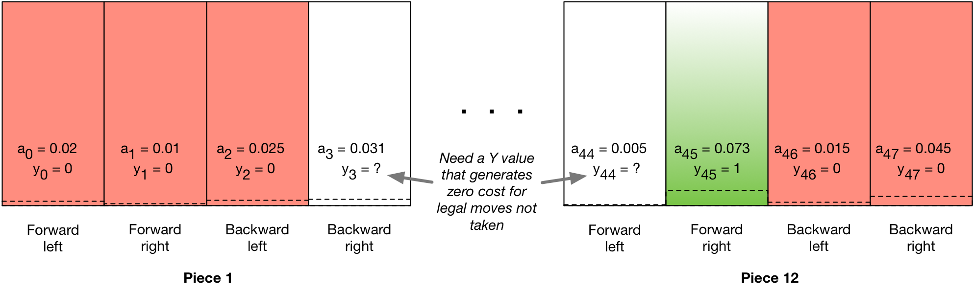
Using a zero-cost label value for that output will generate a 0 gradient for that output during backdrop, and thus not push any associated weights or biases up or down. We can figure out what the cost would be by looking at the equation as it applies to each output and set it equal to zero:

$$(y_j^{(i)}\log\left(a_j^{[L] (i)}\right) + (1-y_j^{(i)})\log\left(1-a_j^{[L](i)}\right)) = 0$$

Solving for \(y_j^{(i)}\) gives us:

$$y_j^{(i)} = \frac{-\log(1-a_j^{[L](i)})}{\log( a_j^{[L](i)})-\log(1-a_j^{[L](i)})}$$

So we’re set, right? Unfortunately, here’s the graph of that function:

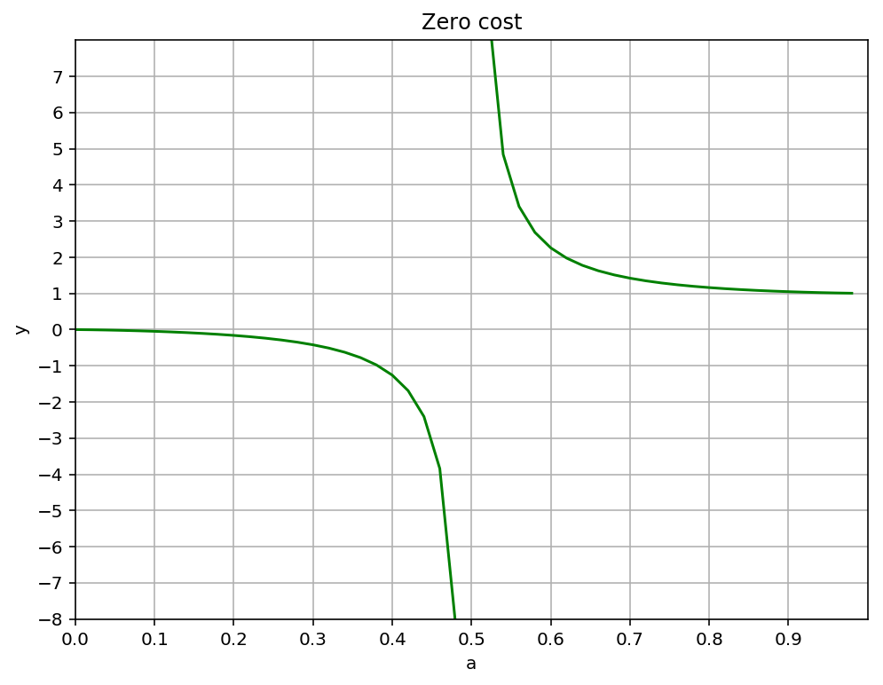
Two important things to note. First and most important, except for \(a = 0\) and \(a = 1\), the zero-cost values for \(y\) are always either greater than one or less than zero. Second, there’s a discontinuity at \(a = 0.5\) where \(y\) becomes undefined.

While it’s possible neither of these facts would be deal breakers in practice, the gradients produced by \(a\) values near 0.5 would be huge, and probably not great for the stability of the weights. More importantly, it seems intuitively clear that if you were designing a cost function for the purpose I’m using it for, categorical cross-entropy quite simply isn’t the cos function that you’d design. So I’m not going to use it.

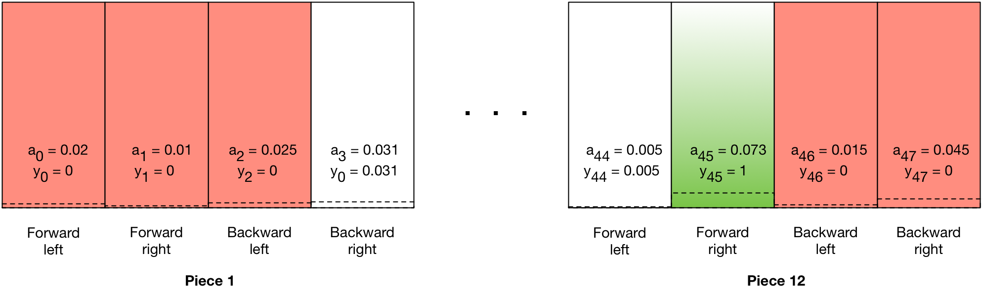
I’m going to use mean squared error, just like it says on the tin. Using that, zero cost becomes simple. Simply set \(y = a\) and you have a zero gradient, and training won’t touch any of the weights connected to those outputs.

Easy peasy lemon squeezy.