Softmax Back Propagation Solved (I think)
Note: This post is the ultimate result of my quest for how to do softmax backpropagation in my hand-coded model for this project. The actual math for softmax back propagation is not something that was specifically covered in my coursework. Furthermore, it’s not something that was easy to Google the answer for since the vast majority of resources on this pair the softmax back propagation fairly inextricably with a cross-entropy cost function, rather than MSE which I’ve used. Thus, it was a significant endeavor to figure out how to do that backprop. This is the result.
I think I’ve finally solved my softmax back propagation gradient. For starters, let’s review the results of the gradient check. When I would run the gradient check on pretty much anything (usually sigmoid output and MSE cost function), I’d get a difference something like \(5.3677365733335105\times 10^{\ -08}\). However, for anything I did with softmax, a typical gradient check would generate a difference like \(0.6593782043630477\). That’s 10 million times larger than it should be.
Here’s the blow-by-blow of how that got solved.
The Wrong Answer
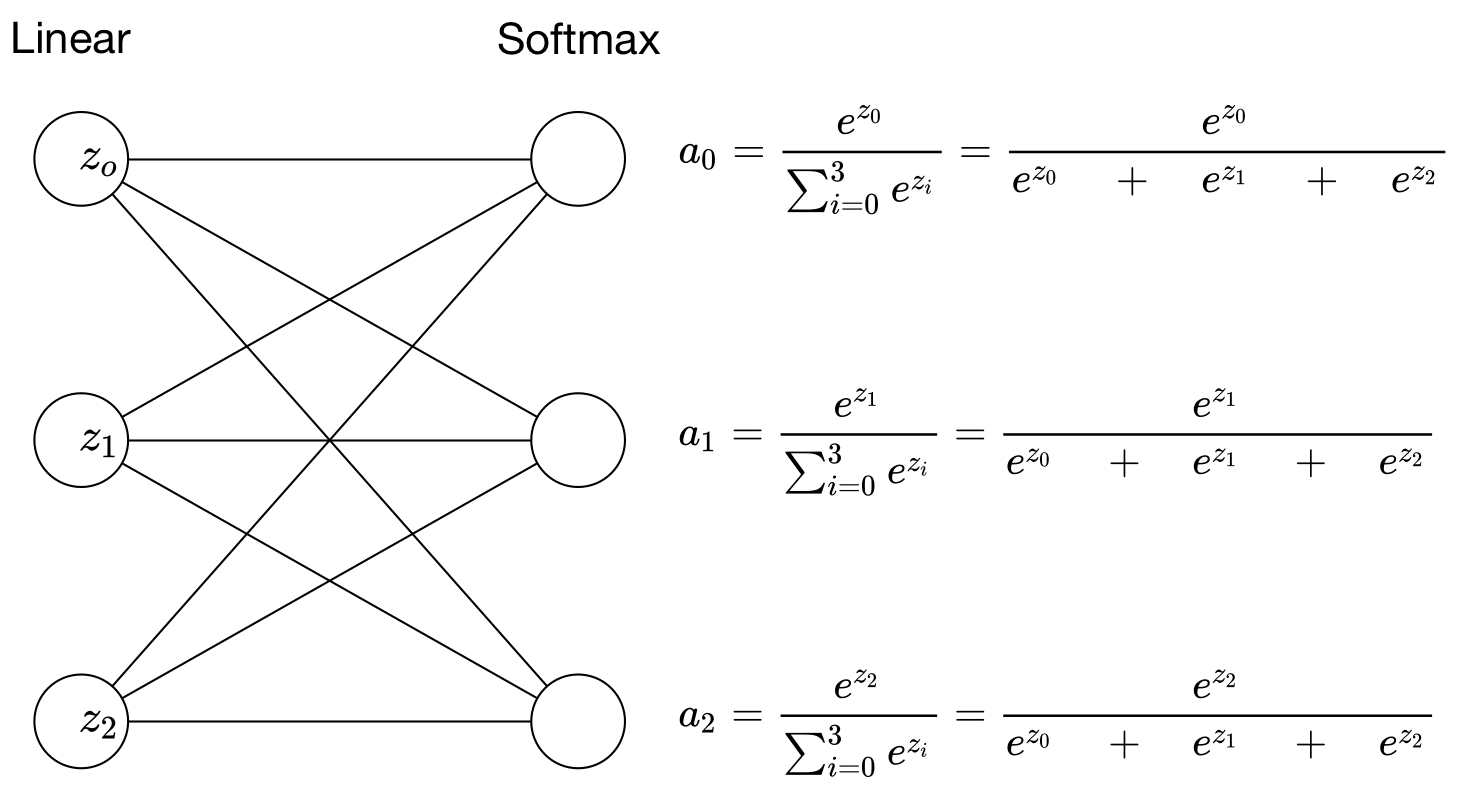
As I mentioned, I had been using the same derivative for softmax as one would use for sigmoid. It was wrong, but here’s why I thought it was right. To get very concrete, we can start by looking at a much smaller 3 output linear/softmax layer:

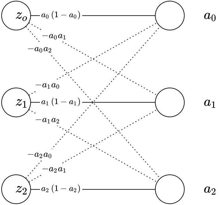
If we’re going to get gradients for the \(W\) and \(b\) parameters that generate each of our \(z\) linear outputs, first we need \(\frac{∂{a}}{∂{z}}\) for all components \(z_{i}\). Because, unlike sigmoid, the each nonlinear output \(a_{j}\) is dependent upon all components of \(z\), the derivative is the following Jacobian matrix:

Visually, this maps to:

My original assumption had been that since I’m trying to get to \(\frac{∂L}{∂z_{0}}, \frac{∂L}{∂z_{1}},\) and \(\frac{∂L}{∂z_{2}}\), I was assuming that I could just use:
$$\frac{∂L}{∂z_{0}}=\frac{∂a_{0}}{∂z_{0}}\frac{∂L}{∂a_{0}}$$
$$\frac{∂L}{∂z_{1}}=\frac{∂a_{1}}{∂z_{1}}\frac{∂L}{∂a_{1}}$$
$$\frac{∂L}{∂z_{2}}=\frac{∂a_{2}}{∂z_{2}}\frac{∂L}{∂a_{2}}$$
Essentially, I was thinking I only needed to account for the solid lines in the above diagram, meaning I only care about:
\(\frac {∂ L }{∂ z_{ i } } =\frac {∂ a_{ j } }{∂ z_{ i } }\frac {∂ L }{∂ a_{ j } } \) for \(i = j\). And thus \(\frac {∂ a_{ j=i } }{∂ z_{ i } } = a_{ j=i }(1-a_{ j=i }) = a_{ i }(1-a_{ i })\). Which translates to
$$\frac{∂L}{∂z_{0}}= a_{ 0 }(1-a_{ 0 })$$
$$\frac{∂L}{∂z_{1}}= a_{ 1 }(1-a_{ 1 })$$
$$\frac{∂L}{∂z_{2}}= a_{ 2 }(1-a_{ 2 })$$
Sigmoid derivative!
Wrong!
The Right Answer
My gradient check told me unambiguously that this was not the correct derivative. So I figured that somehow, the other elements of that Jacobian matrix needed to be accounted for. But ultimately, for each component \(z_{i}\), I need a scalar derivative value, so somehow, I needed to figure out how to take the right side of the equation below and convert to a scalar:

The first, and most obvious thing that occurred to me was close, but wrong. It was to sum them like so:
$$\frac { ∂{ a } }{ ∂{ { { z }_{ i } } } } =\sum _{ j=0 }^{ T } \frac { ∂{ a }_{ j } }{ ∂{ z }_{ i } }$$
and then ultimately, I’d multiply element-wise by the cost derivative to get:
$$\frac{∂L}{∂z_{i}}=\frac{∂a}{∂z_{i}}\frac{∂L}{∂a}$$
The problem is that $$\sum _{ j=0 }^{ T } \frac { ∂{ a }_{ j } }{ ∂{ z }_{ i } } = { a }_{ i }-{ a }_{ i }*\left( \sum _{ j=0 }^{ T } a_{ j } \right)$$ And since \(\sum _{ j=0 }^{ T } a_{ j } = 1\), $$\frac { ∂{ a } }{ ∂{ { { z }_{ i } } } } ={ a }_{ i }-{ a }_{ i }*\left( \sum _{ j=0 }^{ T } a_{ j } \right) ={ a }_{ i }-{ a }_{ i }*\left( 1 \right) =0$$
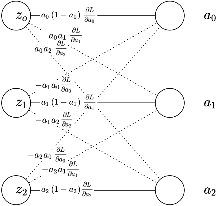
So that’s not going to work. But then, it occurred to me that if you’re going to use all the discrete \(a_{i}\) components, rather than multiplying the cumulative \(\frac { ∂{ a } }{ ∂{ { { z }_{ i } } } }\) by the cumulative \(\frac { ∂{ L } }{ ∂{ {a } } }\), instead we should break each into components, multiply together, and then take the sum of the multiplied components. Here it is visually:

So then, if we take this specific softmax Jacobian derivative matrix:

and multiply the appropriate output column \(j\) by that component of the cost derivative, we get:

Then, if we take the sums of each row, we get:

At this point, we can safely generalize:
$$\frac { ∂L }{ ∂{ z }_{ i } } ={ a }_{ i }\left( \frac { ∂{ L } }{ ∂{ { { a }_{ i } } } } -{ \left( \frac { ∂{ L } }{ ∂{ { { a } } } } \right) }^{ T }\cdot { { a } } \right) $$
Voila!
In Python, here’s how that ends up looking:
def softmax_backward(dA, cache):
"""
Implement the backward propagation for a single SOFTMAX unit.

Arguments:
dA -- post-activation gradient, of any shape
cache -- I store 'Z' for computing backward propagation efficiently

Returns:
dZ -- Gradient of the cost with respect to Z
"""

Z = cache

exps = np.exp(Z)
a = exps / np.sum(exps, axis = 0, keepdims=True)

dA_a = np.sum(dA * a, axis = 0)

dZ = a * (dA - dA_a)

return dZ
Note, I didn’t actually use dot product for \({ \left( \frac { ∂{ L } }{ ∂{ { { a } } } } \right) }^{ T }\cdot { { a } }\). That only works for a single training example. Since I’m using batch training, I just did element wise multiplication across all components and training examples and then summed the components of each training example.
And now, with my new softmax back propagation algorithm, when I run the gradient check, I get \(5.526314030631252 \times 10^{\ -07}\). It’s an order of magnitude larger than what I get for sigmoid, but it’s also a fundamentally different gradient calculation. So even though it’s above the threshold the gradient checker considers to be a mistake in the gradient, the checker and its threshold was written for sigmoid. Given that it’s literally one millionth what the previous gradient difference is, I think I’m implementing it correctly.
Unfortunately, being able to use softmax correctly didn’t in any way magically make my network stop having all that erratic behavior as training went on. I’m not going to write about that now, though. I’m tired and I need to get to bed.